Verification example
In this example, we investigate the verification example from the xARPES manuscript examples section.
This example corresponds to the “Verification using model data” Section from the first xARPES publication: https://www.nature.com/articles/s41524-026-02026-9, going through all the steps discussed in the main text. The notebook also contains an execution of the Bayesian loop with a set of parameters that is “far from” the optimal solution, similar to the supplemental section on the example.
In the future, functionality will be added to xARPES for users to generate their own mock example, allowing for testing of desired hypotheses.
First, we set the desired graphical environment, load xARPES and packages that we will use directly, and set the default xARPES plotting environment.
[ ]:
%load_ext autoreload
%autoreload 2

# Necessary packages
import xarpes
import numpy as np
import matplotlib.pyplot as plt
import os

# Default plot configuration from xarpes.plotting.py
xarpes.plot_settings('default')
The autoreload extension is already loaded. To reload it, use:
  %reload_ext autoreload
We detect the folder in which this file is called, and we set its relevant subfolders.
[ ]:
script_dir = xarpes.set_script_dir()

dfld = 'data_sets'           # Folder containing the data
flnm = 'artificial_einstein' # Name of the file
We load the simulated angles (angl), kinetic energies (ekns), and photoemission intensities (intn) to construct the band map for the artificial example.
[ ]:
angl = np.load(os.path.join(script_dir, dfld, "verification_angles.npy"))
ekns = np.load(os.path.join(script_dir, dfld, "verification_kinergies.npy"))
intn = np.load(os.path.join(script_dir, dfld, "verification_intensities.npy"))
These data are combined with an energy resolution \(\Delta E =2.5\,\mathrm{meV}\), an angular resolution of \(\Delta \eta=0.1^{\circ}\), for a band map at \(T = 10\,\mathrm{meV}\).
For the plotting, abscissa can be changed from angle to momentum (representing the wavevector). After the Fermi-edge fit (see next step), ordinate can also be changed from kinetic_energy to binding_energy.
At any point, you can learn more about the functionality of the xARPES code with commands such as help(bmap.plot).
[ ]:
%matplotlib inline

fig = plt.figure(figsize=(8, 5)); ax = fig.gca()

bmap = xarpes.BandMap.from_np_arrays(intensities=intn, angles=angl, ekin=ekns,
        energy_resolution=0.0025, angle_resolution=0.1, temperature=10)

fig = bmap.plot(abscissa='angle', ordinate='kinetic_energy', ax=ax)
As the first step in the xARPES workflow (https://www.nature.com/articles/s41524-026-02026-9 Fig. 2), we fit the Fermi edge from the angle-integrated photointensity \(\widetilde{P}(E^{\mathrm{kin}})\).
This results in the estimate of the photon energy \(h\widehat{\nu}\) minus the work function \(\widehat{\Phi}\). A full description of the procedure is provided in “Fermi-edge fit” in the Methods section of the publication.
[ ]:
%matplotlib inline

fig = plt.figure(figsize=(6, 5)); ax = fig.gca()

fig = bmap.fit_fermi_edge(hnuminPhi_guess=30, background_guess=1e4,
                          integrated_weight_guess=3e4, angle_min=-6,
                          angle_max=10, ekin_min=29.99, ekin_max=30.02,
                          ax=ax, show=True, fig_close=True,
                          title='Fermi edge fit')

print('The optimised hnu - Phi=' + f'{bmap.hnuminPhi:.4f}' + ' +/- '
      + f'{1.96 * bmap.hnuminPhi_std:.5f}' + ' eV.')
The optimised hnu - Phi=29.9999 +/- 0.00002 eV.
As the second step, the fitting of the MDC maxima is performed.
This step requires setting the minimum and maximum (\(2^\circ\) to \(10^\circ\)) for the angle \(\eta\), the range (\(-80\,\mathrm{meV}\) to \(0.1\,\mathrm{meV}\)) for the binding energy \(E-\mu\), and the band extremum \(k^{\mathrm{c}}=0.1\,\)Å\(^{-1}\). Afterwards, the result at the slice closest to the selected binding energy \(E-\mu\,=0\) is displayed.
Note that the peak is \(5.1^{\circ}\) away from the center, corresponding to about \(2^{\circ}\) at the selected binding energy. xARPES allows for specifying the extremum either as a wavevector or as an angle, whichever is found to be most convenient. This can be seen by uncommenting the SpectralQuadratic definition with the angle and commenting the definition with the wavevector.
[ ]:
%matplotlib inline

angle_min = 2
angle_max = 10

energy_range = [-0.08, 0.0001]
energy_value = 0.0

k_0 = 0.1

mdcs = xarpes.MDCs(*bmap.mdc_set(angle_min, angle_max, energy_range=energy_range))

guess_dists = xarpes.CreateDistributions([
xarpes.Constant(offset=40),
xarpes.SpectralQuadratic(amplitude=0.25, peak=5.1, broadening=0.0005,
            center_wavevector=k_0, name='Right_branch', index='1')
# xarpes.SpectralQuadratic(amplitude=0.25, peak=5.1, broadening=0.0005,
#             center_angle=2.0, name='Right_branch', index='1')
])

fig = plt.figure(figsize=(8, 6)); ax = fig.gca()

fig = mdcs.visualize_guess(distributions=guess_dists, energy_value=energy_value, ax=ax)
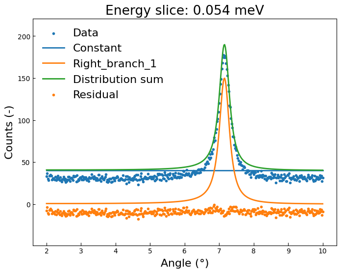
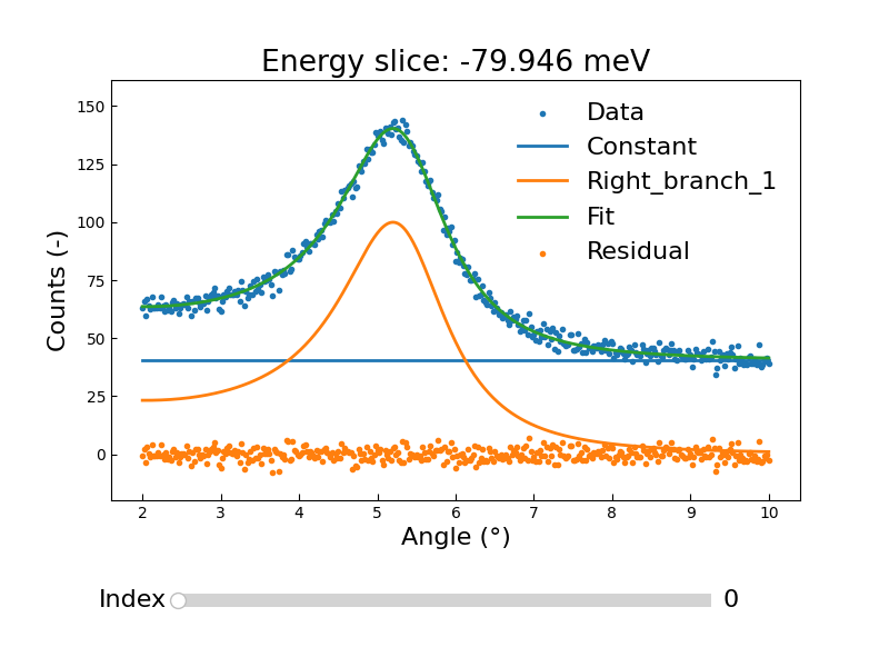
In the following cell, the selected set of MDCs is fitted, after which an interactive figure with a slider is generated. by sliding through the MDCs, you should find that the asymmetry increases towards the bottom of the parabola.
Note on interactive figures
The interactive figure might not work inside the Jupyter notebooks, despite our best efforts to ensure stability.
As a fallback, the user may switch from “%matplotlib widget” to “%matplotlib qt”, after which the figure should pop up in an external window.
For some package versions, a static version of the interactive widget may spuriously show up inside other cells. This undesired behaviour may be circumvented by (once again) executing
xarpes.plot_settings('default').
[ ]:
%matplotlib widget

fig = plt.figure(figsize=(8, 6)); ax = fig.gca()

fig = mdcs.fit_selection(distributions=guess_dists, ax=ax)

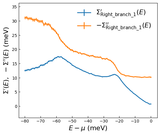
First, we calculate the real \(\widetilde{\Sigma}_{n0}^{\prime}(E_j)\) and minus imaginary parts \(-\widetilde{\Sigma}_{n0}^{\prime\prime}(E_j)\) of the one-shot self-energy, using the right-hand branch as a first example.
Following the section ‘’Extraction of the self-energy” of the publication, this calculation requires a one-shot initial guess for the bare mass \(m_{n0}^{\mathrm{b}}\) and the Fermi wavevector \(k_{n0}^{\mathrm{F}}\). We will use the Bayesian loop to optimise these parameters later on. However, the loop requires a sufficiently good initial guess of these parameters. Therefore, the following plot is useful for improving the initial guess.
[ ]:
%matplotlib inline

fig = plt.figure(figsize=(6, 5)); ax = fig.gca()

self_energy = xarpes.SelfEnergy(*mdcs.expose_parameters(select_label='Right_branch_1',
                                bare_mass=1.59675179, fermi_wavevector=0.2499758715, side='right'))

fig = self_energy.plot_both(ax=ax, scale='meV')

plt.show()
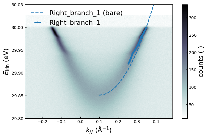
Having completed the MDC fitting procedure, we can plot the MDC maxima \(\widetilde{k}(E_j)\) on top of the band map.
Given the (initial guess) for the bare-band parameters, we can plot the bare band on top of the band map as well.
Given abscissa='momentum', a warning is printed as a reminder there is warping associated with going from angular space to momentum space.
You can have a look at the different options for plot_dispersions: full, none, kink, and domain.
[ ]:
%matplotlib inline

self_energies = xarpes.CreateSelfEnergies([self_energy])

fig = plt.figure(figsize=(8, 5)); ax = fig.gca()

ax.set_ylim(29.8, 30.05)

fig = bmap.plot(abscissa='momentum', ordinate='kinetic_energy',
                plot_dispersions='domain', self_energies=self_energies, ax=ax)
/home/tvanwaas/projects/xARPES/xarpes/plotting.py:72: UserWarning: Conversion from angle to momenta causes warping of the cell centers.
 Cell edges of the mesh plot may look irregular.
  result = func(*args, **kwargs)
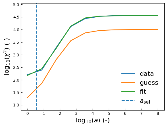
‘’Chi2kink method’’
In the following cell, we extract the Eliashberg function from the self-energy. This extraction is based on the maximum-entropy method. We have chosen the chi2kink flavour of the maximum-entropy method. Accordingly, the result of the chi2kink fit is plotted during the extraction. Setting show=False and fig_close=True will prevent the figure from being displayed. Afterwards, we plot the Eliashberg function and model function with the appropriate self-energy methods.
To model the characteristic kink-like behavior observed in the dependence of the goodness-of-fit metric on the control parameter \(x\), we employ a smooth logistic function, hereafter referred to as the \(\chi^2\)-kink model. The fitted function is defined as
where \(g\) denotes the asymptotic baseline value of the metric for small \(x\), \(b\) sets the amplitude of the step, \(c\) determines the position of the kink along the \(x\)-axis, and \(d\) controls the sharpness of the transition. Once the fitting has been completed, the selected \(a_{\mathrm{sel}}\) is obtained from \(a=10^{c-f /d}\) with a tuning parameter \(f \in [2, 2.5]\).
For a full description of the ‘’chi2kink’’ method, please see https://doi.org/10.1016/j.cpc.2022.108519.
Extraction of the Eliashberg function
There are many parameters involved in the extraction of \(\alpha^2F_n(\omega)\). The energies encountered in supplemental section ‘’Details on the Eliashberg-function extraction’’ are identified as omega_min, omega_max, omega_I, omega_M, and omega_S, discretising \(m_n(\omega)\) with omega_num points. aval_min, aval_max, and aval_num describe the discretisation of the ‘’chi2kink’’ interval, with initial guesses g_guess, b_guess, c_guess,
and d_guess. Finally, initial guesses for \(\lambda_n^{\mathrm{el}}\), \(\Gamma_n^{\mathrm{imp}}\), and \(h_n\) can be provided as lambda_el, impurity_magnitude, and h_n, respectively.
[ ]:
%matplotlib inline

fig, spectrum, model, omega_range, aval_select = self_energy.extract_a2f(
    omega_min=1.0, omega_max=80, omega_num=250, omega_I=20, omega_M=60,
    aval_min=1.5, aval_num=10, aval_max=9.5, lambda_el=0.1132858,
    impurity_magnitude=10.041243, h_n=0.0803366,
    g_guess=1.0, b_guess=3.0, c_guess=3.0, d_guess=1.5,
    show=True, fig_close=False)

plt.show()
Dimensionality has been reduced from a matrix of rank 156 to 122 in the singular space.
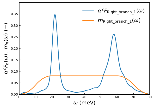
The Eliashberg function and model function
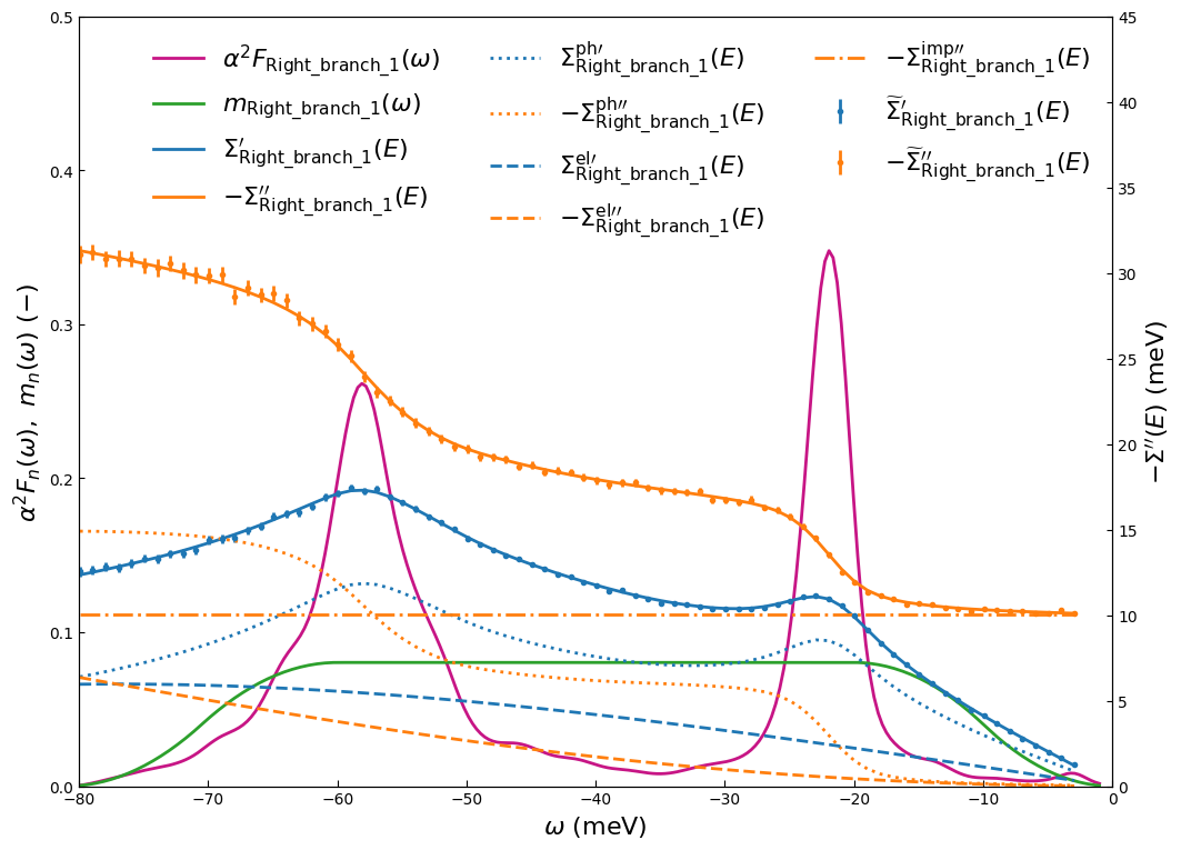
Having performed the one-shot extraction, we can inspect the Eliashberg function and the associated model function \(m_n(\omega)\) that we used as part of the maximum-entropy method.
[ ]:
%matplotlib inline

fig = plt.figure(figsize=(7, 5)); ax = fig.gca()

fig = self_energy.plot_spectra(ax=ax)

plt.show()
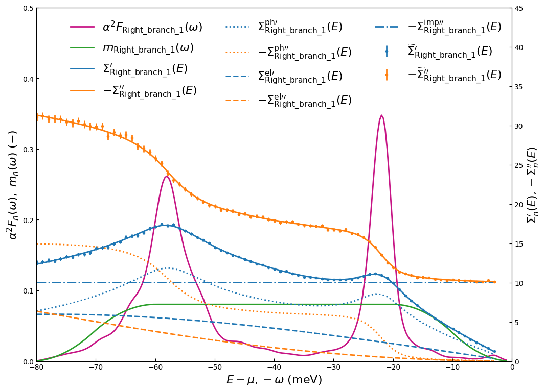
The following plots all of the extracted quantities in a single figure. The figure also showcases typical xARPES usage: start with some generic xarpes functionalities such as plot_spectra, then tailor the plotted output towards the desired output, such as for scientific presentations/publications.
The following figure shows not just the spectra from the previous figure, but it also decomposes the self-energy into the electron-phonon \(\Sigma_{n}^{\mathrm{ph}}(E)\), electron-electron \(\Sigma_{n}^{\mathrm{el}}(E)\), and electron-impurity \(\Sigma_{n}^{\mathrm{imp}}(E)\) contributions. After this one-shot calculation, we will have a look at how to quantify these latter two contributions using the Bayesian loop.
By default, The Eliashberg function is extracted while removing the self-energies for binding energies smaller than the energy resolution. For transparency, these self-energies are then also eliminated from the displayed result.
[ ]:
%matplotlib inline

color_one = "tab:blue"; color_two = "tab:orange"
color_three = "mediumvioletred"; color_four = "tab:green"

fig = plt.figure(figsize=(12, 9)); ax1 = fig.add_subplot(111); ax2 = ax1.twinx()

self_energy.plot_spectra(ax=ax1, abscissa="reversed", show=False, fig_close=False)
self_energy.plot_reconstructed_both(ax=ax2, scale="meV", show=False, fig_close=False)
self_energy.plot_reconstructed_both_ph(ax=ax2, scale="meV", linestyle=":",
    show=False, fig_close=False)
self_energy.plot_reconstructed_both_el(ax=ax2, scale="meV", linestyle="--",
    show=False, fig_close=False)
self_energy.plot_reconstructed_imag_imp(ax=ax2, scale="meV", linestyle="-.",
    show=False, fig_close=False)
self_energy.plot_both(ax=ax2, scale="meV", resolution_range="applied", fmt="o",
    show=False, fig_close=False)

# --- Change colours for self-energy lines on ax2
lines = ax2.get_lines()
[line.set_color(color_one) for line in lines[-9:-1:2]]
[line.set_color(color_two) for line in lines[-8:-1:2]]
lines[-2].set_color(color_one); lines[-1].set_color(color_two)

# --- Change colours for error bars from plot_both
real_err, imag_err = ax2.collections[-2:]
real_err.set_color(color_one); imag_err.set_color(color_two)

# --- Change colours for spectra
a2f_line, model_line = ax1.get_lines()[-2:]
a2f_line.set_color(color_three); model_line.set_color(color_four)

#Tiny tweaks that should have been xARPES default behaviour.
ax1.set_xlabel('$E-\mu, -\omega$ (meV)')
ax2.set_ylabel('$\Sigma_{n}^{\prime}(E), -\Sigma_{n}^{\prime\prime}(E)$')

# --- Overwrite the legend with a custom legend
[ax.get_legend() and ax.get_legend().remove() for ax in (ax1, ax2)]
h1, l1 = ax1.get_legend_handles_labels(); h2, l2 = ax2.get_legend_handles_labels()
ax1.legend(h1 + h2, l1 + l2, ncol=3)
ax1.set_ylim([0, 0.5]); ax2.set_ylim([0, 45])

plt.show()
The Bayesian loop
We now turn to the optimisation of the model parameters: The Fermi wavevector \(k_n^{\mathrm{F}}\), the bare mass \(m_n^{\mathrm{b}}\), the electron-electron coupling coefficient \(\lambda_n^{\mathrm{el}}\), and the height of the model function \(h_n\).
For simplicity, we will first start from the optimal solution itself. Thus, the optimisation should effectively return to this solution after a couple tens of iterations. Aside from more forgiving \(a_{\mathrm{min}}\) and \(a_{\mathrm{max}}\) during the optimisation, the only new variables pertain to the relative size in the steps for the model parameters, named scale_mb et cetera. These scaling factors can be modified to ensure the code finds a better solution, while not making
steps so large that the inner MEM loop fails to extract the Eliashberg function.
[ ]:
with xarpes.trim_notebook_output(print_lines=10):
    spectrum, model, omega_range, aval_select, cost, params = self_energy.bayesian_loop(
            omega_min=1.0, omega_max=80, omega_num=250, omega_I=20, omega_M=60,
            aval_min=3.0, aval_max=11.0, bare_mass=1.597636665,
            fermi_wavevector=0.2499774217, h_n=0.081811739,
            impurity_magnitude=10.0379498, lambda_el=0.1054932517,
            vary=("impurity_magnitude", "lambda_el", "fermi_wavevector",
                  "bare_mass", "h_n"),
            scale_mb=0.01, scale_imp=0.1, scale_kF=0.001,
            scale_lambda_el=0.1, scale_hn=0.1)
Dimensionality has been reduced from a matrix of rank 156 to 122 in the singular space.
Iter    1 | cost = -5.1735e+02 | bare_mass=1.5976367 | fermi_wavevector=0.24997742 | h_n=0.081811739 | impurity_magnitude=10.03795 | lambda_el=0.10549325
Iter    2 | cost = -5.1735e+02 | bare_mass=1.5976367 | fermi_wavevector=0.24997742 | h_n=0.081811739 | impurity_magnitude=10.037975 | lambda_el=0.10549325
Iter    3 | cost = -5.1734e+02 | bare_mass=1.5976367 | fermi_wavevector=0.24997742 | h_n=0.081811739 | impurity_magnitude=10.03795 | lambda_el=0.10551825
Iter    4 | cost = -5.1735e+02 | bare_mass=1.5976367 | fermi_wavevector=0.24997767 | h_n=0.081811739 | impurity_magnitude=10.03795 | lambda_el=0.10549325
Iter    5 | cost = -5.1735e+02 | bare_mass=1.5976392 | fermi_wavevector=0.24997742 | h_n=0.081811739 | impurity_magnitude=10.03795 | lambda_el=0.10549325
Iter    6 | cost = -5.1734e+02 | bare_mass=1.5976367 | fermi_wavevector=0.24997742 | h_n=0.081836739 | impurity_magnitude=10.03795 | lambda_el=0.10549325
Iter    7 | cost = -5.1734e+02 | bare_mass=1.5976377 | fermi_wavevector=0.24997752 | h_n=0.081786739 | impurity_magnitude=10.03796 | lambda_el=0.10550325
Iter    8 | cost = -5.1734e+02 | bare_mass=1.5976374 | fermi_wavevector=0.2499775 | h_n=0.081799239 | impurity_magnitude=10.037957 | lambda_el=0.10550075
Iter    9 | cost = -5.1734e+02 | bare_mass=1.5976369 | fermi_wavevector=0.24997745 | h_n=0.081824239 | impurity_magnitude=10.037952 | lambda_el=0.10549575
... (31 lines omitted) ...
Iter   41 | cost = -5.1735e+02 | bare_mass=1.5976373 | fermi_wavevector=0.24997742 | h_n=0.081811516 | impurity_magnitude=10.03796 | lambda_el=0.10549306
Iter   42 | cost = -5.1735e+02 | bare_mass=1.5976368 | fermi_wavevector=0.24997743 | h_n=0.081811765 | impurity_magnitude=10.037961 | lambda_el=0.10549276
Iter   43 | cost = -5.1735e+02 | bare_mass=1.5976373 | fermi_wavevector=0.24997742 | h_n=0.081811421 | impurity_magnitude=10.037959 | lambda_el=0.10549387
Iter   44 | cost = -5.1735e+02 | bare_mass=1.5976369 | fermi_wavevector=0.24997741 | h_n=0.081812025 | impurity_magnitude=10.037962 | lambda_el=0.1054923
Iter   45 | cost = -5.1735e+02 | bare_mass=1.5976376 | fermi_wavevector=0.24997741 | h_n=0.081811555 | impurity_magnitude=10.037941 | lambda_el=0.10549313
Iter   46 | cost = -5.1735e+02 | bare_mass=1.5976369 | fermi_wavevector=0.24997742 | h_n=0.081811693 | impurity_magnitude=10.037966 | lambda_el=0.10549322
Iter   47 | cost = -5.1735e+02 | bare_mass=1.5976374 | fermi_wavevector=0.24997742 | h_n=0.081811135 | impurity_magnitude=10.037955 | lambda_el=0.10549445
Iter   48 | cost = -5.1735e+02 | bare_mass=1.5976373 | fermi_wavevector=0.24997742 | h_n=0.081811358 | impurity_magnitude=10.037957 | lambda_el=0.10549392
Optimised parameters:
bare_mass=1.5976373, fermi_wavevector=0.249977421, h_n=0.08181135793, impurity_magnitude=10.03795677, lambda_el=0.1054939153
If the optimsation works from a trivial starting point, we can also start from a much less probable initial guess, to showcase that the code can also find the final solution, provided that there is some internal consistency among the initial parameters, as discussed in the supplement of the paper.
Note that the optimisation can be slightly sensitive to the combination of Python, NumPy, and Scipy. The following results have been tested against Python v3.10.12, NumPy v2.2.6, and SciPy v1.15.3. The optimisation might get stuck along the way for other combinations.
[ ]:
with xarpes.trim_notebook_output(print_lines=10):
    spectrum, model, omega_range, aval_select, cost, params = self_energy.bayesian_loop(omega_min=1.0,
                omega_max=80, omega_num=250, omega_I=20, omega_M=60,
                aval_min=3.0, aval_max=11.0, bare_mass=1.74625, fermi_wavevector=0.250125,
                h_n=0.09, impurity_magnitude=9.1, lambda_el=0.22, sigma_svd=0.1,
                vary=("impurity_magnitude", "lambda_el", "fermi_wavevector", "bare_mass", "h_n"),
                converge_iters=100, tole=1e-8, scale_mb=0.1, scale_imp=1.0, scale_kF=0.001,
                scale_lambda_el=0.1, scale_hn=0.01)
Dimensionality has been reduced from a matrix of rank 156 to 58 in the singular space.
Iter    1 | cost =  5.3786e+04 | bare_mass=1.74625 | fermi_wavevector=0.250125 | h_n=0.09 | impurity_magnitude=9.1 | lambda_el=0.22
Iter    2 | cost =  5.3786e+04 | bare_mass=1.74625 | fermi_wavevector=0.250125 | h_n=0.09 | impurity_magnitude=9.10025 | lambda_el=0.22
Iter    3 | cost =  5.3808e+04 | bare_mass=1.74625 | fermi_wavevector=0.250125 | h_n=0.09 | impurity_magnitude=9.1 | lambda_el=0.220025
Iter    4 | cost =  5.3779e+04 | bare_mass=1.74625 | fermi_wavevector=0.25012525 | h_n=0.09 | impurity_magnitude=9.1 | lambda_el=0.22
Iter    5 | cost =  5.3806e+04 | bare_mass=1.746275 | fermi_wavevector=0.250125 | h_n=0.09 | impurity_magnitude=9.1 | lambda_el=0.22
Iter    6 | cost =  5.3787e+04 | bare_mass=1.74625 | fermi_wavevector=0.250125 | h_n=0.0900025 | impurity_magnitude=9.1 | lambda_el=0.22
Iter    7 | cost =  5.3770e+04 | bare_mass=1.74626 | fermi_wavevector=0.2501251 | h_n=0.090001 | impurity_magnitude=9.1001 | lambda_el=0.219975
Iter    8 | cost =  5.3751e+04 | bare_mass=1.746265 | fermi_wavevector=0.25012515 | h_n=0.0900015 | impurity_magnitude=9.10015 | lambda_el=0.21995
Iter    9 | cost =  5.3749e+04 | bare_mass=1.746231 | fermi_wavevector=0.25012516 | h_n=0.0900016 | impurity_magnitude=9.10016 | lambda_el=0.21998
... (738 lines omitted) ...
Iter  487 | cost = -5.1735e+02 | bare_mass=1.5976358 | fermi_wavevector=0.2499774 | h_n=0.081810544 | impurity_magnitude=10.03797 | lambda_el=0.10549741
Iter  488 | cost = -5.1735e+02 | bare_mass=1.5976356 | fermi_wavevector=0.24997741 | h_n=0.081810589 | impurity_magnitude=10.037984 | lambda_el=0.10549778
Iter  489 | cost = -5.1735e+02 | bare_mass=1.5976359 | fermi_wavevector=0.24997741 | h_n=0.081810837 | impurity_magnitude=10.037973 | lambda_el=0.10549625
Iter  490 | cost = -5.1735e+02 | bare_mass=1.5976367 | fermi_wavevector=0.2499774 | h_n=0.081811217 | impurity_magnitude=10.037965 | lambda_el=0.10549464
Iter  491 | cost = -5.1735e+02 | bare_mass=1.5976346 | fermi_wavevector=0.2499774 | h_n=0.08181085 | impurity_magnitude=10.037982 | lambda_el=0.1054975
Iter  492 | cost = -5.1735e+02 | bare_mass=1.597637 | fermi_wavevector=0.24997741 | h_n=0.081811187 | impurity_magnitude=10.037963 | lambda_el=0.1054944
Iter  493 | cost = -5.1735e+02 | bare_mass=1.5976366 | fermi_wavevector=0.24997741 | h_n=0.081811333 | impurity_magnitude=10.037943 | lambda_el=0.10549496
Iter  494 | cost = -5.1735e+02 | bare_mass=1.5976369 | fermi_wavevector=0.24997742 | h_n=0.081811538 | impurity_magnitude=10.037922 | lambda_el=0.1054947
Optimised parameters:
bare_mass=1.597636642, fermi_wavevector=0.2499774146, h_n=0.08181133262, impurity_magnitude=10.03794324, lambda_el=0.105494957
Following the recommended procedure, we perform a final optimisation with very tight criteria, for the purpose of further narrowing down the solution.
With tightened aval_min, aval_max, the result gets a tiny bit closer to the true solution for some of the parameters (for the tested combination of packages). We also inrease the number of self-energy data used in the singular value decomposition by increasing sigma_svd, we set a very tight loop optimisation criterion using tole, which must be met for a slightly increased number of converge_iters.
[ ]:
with xarpes.trim_notebook_output(print_lines=10):
    spectrum, model, omega_range, aval_select, cost, params = self_energy.bayesian_loop(omega_min=1.0,
                omega_max=80, omega_num=250, omega_I=20, omega_M=60,
                aval_min=1.0, aval_max=9.0, sigma_svd=1e-4,
                bare_mass=1.597636093, fermi_wavevector=0.2499774208, h_n=0.08181151626,
                impurity_magnitude=10.03795642, lambda_el=0.1054945571,
                vary=("impurity_magnitude", "lambda_el", "fermi_wavevector", "bare_mass", "h_n"),
                converge_iters=100, tole=1e-8, scale_mb=0.1, scale_imp=0.1, scale_kF=0.01,
                scale_lambda_el=0.1, scale_hn=0.1)
Dimensionality has been reduced from a matrix of rank 156 to 122 in the singular space.
Iter    1 | cost = -4.4650e+02 | bare_mass=1.5976361 | fermi_wavevector=0.24997742 | h_n=0.081811516 | impurity_magnitude=10.037956 | lambda_el=0.10549456
Iter    2 | cost = -4.4650e+02 | bare_mass=1.5976361 | fermi_wavevector=0.24997742 | h_n=0.081811516 | impurity_magnitude=10.037981 | lambda_el=0.10549456
Iter    3 | cost = -4.4654e+02 | bare_mass=1.5976361 | fermi_wavevector=0.24997742 | h_n=0.081811516 | impurity_magnitude=10.037956 | lambda_el=0.10551956
Iter    4 | cost = -4.4605e+02 | bare_mass=1.5976361 | fermi_wavevector=0.24997992 | h_n=0.081811516 | impurity_magnitude=10.037956 | lambda_el=0.10549456
Iter    5 | cost = -4.4647e+02 | bare_mass=1.5976611 | fermi_wavevector=0.24997742 | h_n=0.081811516 | impurity_magnitude=10.037956 | lambda_el=0.10549456
Iter    6 | cost = -4.4665e+02 | bare_mass=1.5976361 | fermi_wavevector=0.24997742 | h_n=0.081836516 | impurity_magnitude=10.037956 | lambda_el=0.10549456
Iter    7 | cost = -4.4692e+02 | bare_mass=1.5976461 | fermi_wavevector=0.24997492 | h_n=0.081821516 | impurity_magnitude=10.037966 | lambda_el=0.10550456
Iter    8 | cost = -4.4721e+02 | bare_mass=1.5976511 | fermi_wavevector=0.24997242 | h_n=0.081826516 | impurity_magnitude=10.037971 | lambda_el=0.10550956
Iter    9 | cost = -4.4693e+02 | bare_mass=1.5976171 | fermi_wavevector=0.24997542 | h_n=0.081827516 | impurity_magnitude=10.037972 | lambda_el=0.10551056
... (252 lines omitted) ...
Iter  196 | cost = -5.1366e+02 | bare_mass=1.5969085 | fermi_wavevector=0.24997471 | h_n=0.095103288 | impurity_magnitude=10.038144 | lambda_el=0.10606748
Iter  197 | cost = -5.1366e+02 | bare_mass=1.5968905 | fermi_wavevector=0.24997464 | h_n=0.095105263 | impurity_magnitude=10.038143 | lambda_el=0.1060685
Iter  198 | cost = -5.1366e+02 | bare_mass=1.596917 | fermi_wavevector=0.24997469 | h_n=0.095103875 | impurity_magnitude=10.038144 | lambda_el=0.10606651
Iter  199 | cost = -5.1366e+02 | bare_mass=1.596922 | fermi_wavevector=0.24997471 | h_n=0.095101154 | impurity_magnitude=10.038145 | lambda_el=0.10606702
Iter  200 | cost = -5.1366e+02 | bare_mass=1.5969202 | fermi_wavevector=0.24997477 | h_n=0.095110791 | impurity_magnitude=10.038144 | lambda_el=0.10606714
Iter  201 | cost = -5.1366e+02 | bare_mass=1.5969112 | fermi_wavevector=0.24997466 | h_n=0.095101254 | impurity_magnitude=10.038144 | lambda_el=0.10606702
Iter  202 | cost = -5.1366e+02 | bare_mass=1.596902 | fermi_wavevector=0.24997467 | h_n=0.095107751 | impurity_magnitude=10.038143 | lambda_el=0.10606711
Iter  203 | cost = -5.1366e+02 | bare_mass=1.596917 | fermi_wavevector=0.2499747 | h_n=0.095102803 | impurity_magnitude=10.038144 | lambda_el=0.10606704
Optimised parameters:
bare_mass=1.596911184, fermi_wavevector=0.2499746609, h_n=0.09510125354, impurity_magnitude=10.03814392, lambda_el=0.106067022
Once you are done
Once you have finished, there are many things you can try. For example, you could try to repeat the above procedure for the left-hand branch. You will have to find a sufficiently good initial guess for the left-hand Fermi wavevector for the extraction to succeed.
Afterwards, you can move on to the other available xARPES examples. We recommend doing the graphene tutorial as the first tutorial using real experimental data. The graphene tutorial uses a linearised bare band, which is a very common approximation the analysis of many-body quantities from ARPES, although it is a fairly good approximation in graphene. After that tutorial, you could move on to the \(\rm{SrTiO}_3\) tutorial, which showcases the use of heuristically obtained photoemission matrix elements, while quantifying the electronic spectral function \(A_n(E,k_{\parallel})\).