SrTiO3
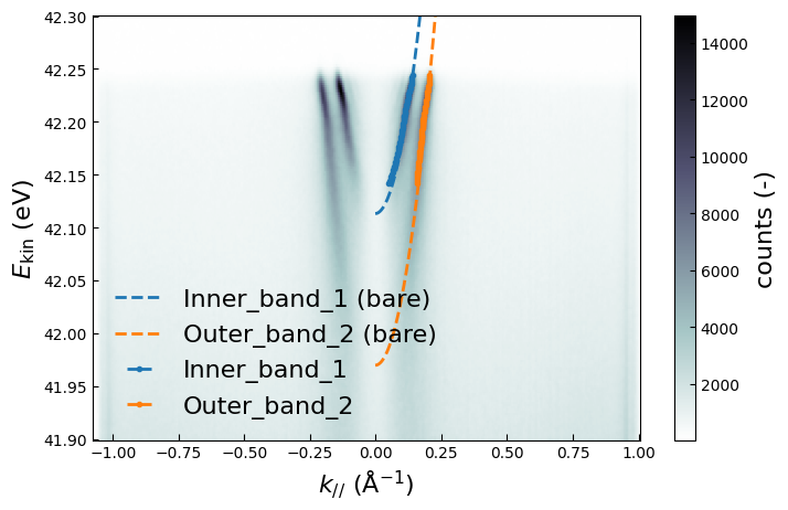
In this example, we extract the self-energies and Eliashberg function from a 2DEL in the \(d_{xy}\) bands on the \(\rm{TiO}_{2}\)-terminated surface of \(\rm{SrTiO}_3\).
[ ]:
%load_ext autoreload
%autoreload 2

# Necessary packages
import xarpes
import matplotlib.pyplot as plt
import os

# Default plot configuration from xarpes.plotting.py
xarpes.plot_settings('default')
[ ]:
script_dir = xarpes.set_script_dir()

dfld = 'data_sets' # Folder containing the data
flnm = 'STO_2_0010STO_2_' # Name of the file
extn = '.ibw' # Extension of the file

data_file_path = os.path.join(script_dir, dfld, flnm + extn)
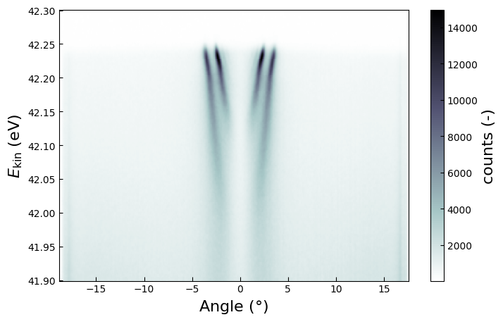
The following cell instantiates band map class object based on the Igor Binary Wave (ibw) file. The subsequent cell illustrates how a band map object could be instantiated with NumPy arrays instead. Only one of the cells will have to be executed to populate the band map object.
[ ]:
%matplotlib inline

fig = plt.figure(figsize=(8, 5)); ax = fig.gca()

bmap = xarpes.BandMap.from_ibw_file(data_file_path, energy_resolution=0.01,
                      angle_resolution=0.2, temperature=20)

bmap.shift_angles(shift=-0.57)

fig = bmap.plot(abscissa='angle', ordinate='kinetic_energy', ax=ax)
[ ]:
# %matplotlib inline

# import numpy as np

# intensities= np.load(os.path.join(dfld, "STO_2_0010STO_2_intensities.npy"))
# angles = np.load(os.path.join(dfld, "STO_2_0010STO_2_angles.npy"))
# ekin = np.load(os.path.join(dfld, "STO_2_0010STO_2_ekin.npy"))

# bmap = xarpes.BandMap.from_ibw_file(data_file_path, energy_resolution=0.01,
#                       angle_resolution=0.2, temperature=20)

# bmap.shift_angles(shift=-0.57)

# fig = plt.figure(figsize=(8, 5)); ax = fig.gca()

# fig = bmap.plot(abscissa='angle', ordinate='kinetic_energy', ax=ax)
[ ]:
%matplotlib inline

fig = bmap.fit_fermi_edge(hnuminPhi_guess=42.24, background_guess=1e4,
                          integrated_weight_guess=1e6, angle_min=-5,
                          angle_max=5, ekin_min=42.22, ekin_max=42.3,
                          show=True, title='Fermi edge fit')

print('The optimised h nu - Phi = ' + f'{bmap.hnuminPhi:.4f}' + ' +/- '
      + f'{bmap.hnuminPhi_std:.4f}' + ' eV.')
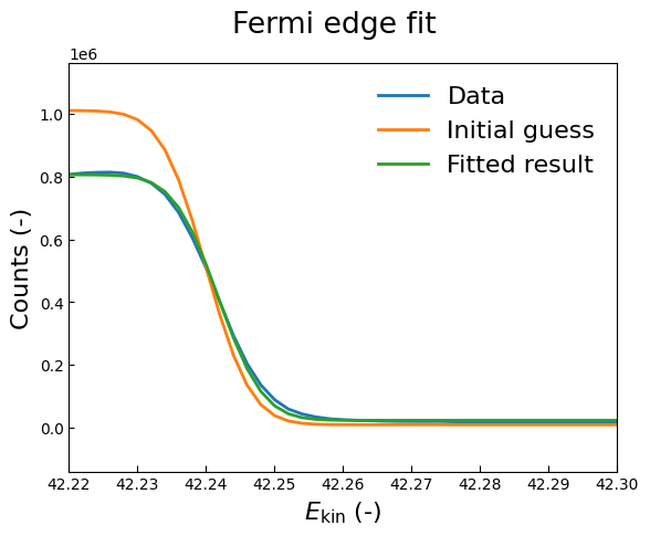
The optimised h nu - Phi = 42.2418 +/- 0.0001 eV.
[ ]:
%matplotlib inline
k_0 = -0.0014 # 0.02
theta_0 = 0
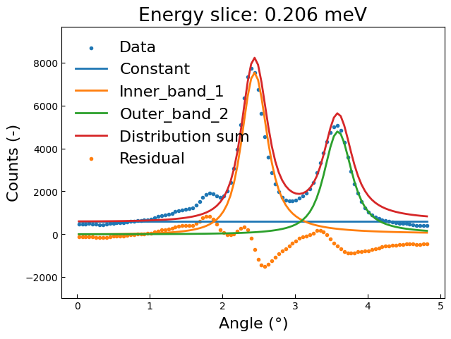
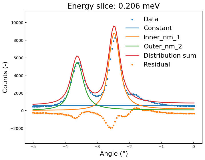
guess_dists = xarpes.CreateDistributions([
xarpes.Constant(offset=600),
xarpes.SpectralQuadratic(amplitude=3800, peak=-2.45, broadening=0.00024,
center_wavevector=k_0, name='Inner_band', index='1'),
xarpes.SpectralQuadratic(amplitude=1800, peak=-3.6, broadening=0.0004,
center_wavevector=k_0, name='Outer_band', index='2')
])
import numpy as np
mat_el = lambda x: np.sin(np.deg2rad(x - theta_0)) ** 2
mat_args = {}
energy_range = [-0.1, 0.003]
angle_min = 0.0
angle_max = 4.8
mdcs = xarpes.MDCs(*bmap.mdc_set(angle_min, angle_max, energy_range=energy_range))
fig = plt.figure(figsize=(7, 5)); ax = fig.gca()
fig = mdcs.visualize_guess(distributions=guess_dists, matrix_element=mat_el,
matrix_args=mat_args, energy_value=-0.000, ax=ax)
Note on interactive figures
The interactive figure might not work inside the Jupyter notebooks, despite our best efforts to ensure stability.
As a fallback, the user may switch from “%matplotlib widget” to “%matplotlib qt”, after which the figure should pop up in an external window.
For some package versions, a static version of the interactive widget may spuriously show up inside other cells. In that case, uncomment the #get_ipython()… line in the first cell for your notebooks.
[ ]:
%matplotlib widget

fig = plt.figure(figsize=(8, 6)); ax = fig.gca()

fig = mdcs.fit_selection(distributions=guess_dists, matrix_element=mat_el,
                         matrix_args=mat_args, ax=ax)

Note on the self-energy assignment
The user has to explicitly assign the peaks as left-hand or right-hand side.
In theory, one could incorporate such information in a minus sign of the peak position.
However, this would also require setting boundaries for the fitting range.
Instead, the user is advised to carefully check correspondence of peak maxima with MDC fitting results.
[ ]:
self_energy = xarpes.SelfEnergy(*mdcs.expose_parameters(select_label='Inner_band_1',
                                bare_mass=0.58997502, fermi_wavevector=0.1411192, side='right'))

self_two = xarpes.SelfEnergy(*mdcs.expose_parameters(select_label='Outer_band_2',
                                bare_mass=0.6, fermi_wavevector=0.207))

self_two.side='right'
[ ]:
%matplotlib inline

self_energies = xarpes.CreateSelfEnergies([self_energy, self_two])

fig = plt.figure(figsize=(8, 5)); ax = fig.gca()

fig = bmap.plot(abscissa='momentum', ordinate='kinetic_energy',
                plot_dispersions='domain',
                self_energies=self_energies, ax=ax)
/home/tvanwaas/projects/xARPES/xarpes/plotting.py:72: UserWarning: Conversion from angle to momenta causes warping of the cell centers.
 Cell edges of the mesh plot may look irregular.
  result = func(*args, **kwargs)
[ ]:
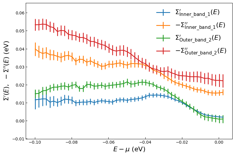
%matplotlib inline

fig = plt.figure(figsize=(9, 6)); ax = fig.gca()

self_energy.plot_both(ax=ax, show=False, fig_close=False)
self_two.plot_both(ax=ax, show=False, fig_close=False)

plt.legend(); plt.show()
[ ]:
%matplotlib inline

guess_dists = xarpes.CreateDistributions([
xarpes.Constant(offset=600),

xarpes.SpectralQuadratic(amplitude=8, peak=2.45, broadening=0.00024,
            center_wavevector=k_0, name='Inner_nm', index='1'),

xarpes.SpectralQuadratic(amplitude=8, peak=3.6, broadening=0.0004,
            center_wavevector=k_0, name='Outer_nm', index='2')
])

energy_range = [-0.1, 0.003]
angle_min=-5.0
angle_max=0.0

mdcs = xarpes.MDCs(*bmap.mdc_set(angle_min, angle_max, energy_range=energy_range))

fig = plt.figure(figsize=(8, 6)); ax = fig.gca()

fig = mdcs.visualize_guess(distributions=guess_dists, ax=ax, energy_value=0)
[ ]:
%matplotlib widget

fig = plt.figure(figsize=(8, 6)); ax = fig.gca()

fig = mdcs.fit_selection(distributions=guess_dists, ax=ax)

[ ]:
self_three = xarpes.SelfEnergy(*mdcs.expose_parameters(select_label='Inner_nm_1', side='left',
                                bare_mass=0.5, fermi_wavevector=0.142))

self_four = xarpes.SelfEnergy(*mdcs.expose_parameters(select_label='Outer_nm_2', side='left',
                                bare_mass=0.62, fermi_wavevector=0.207))
[ ]:
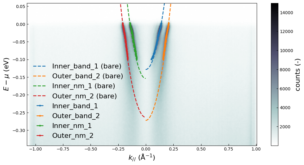
%matplotlib inline

fig = plt.figure(figsize=(12, 6))
ax = fig.gca()

self_total = xarpes.CreateSelfEnergies([
    self_energy, self_two,
    self_three, self_four
])

fig = bmap.plot(abscissa='momentum', ordinate='electron_energy', ax=ax,
                self_energies=self_total, plot_dispersions='domain')
/home/tvanwaas/projects/xARPES/xarpes/plotting.py:72: UserWarning: Conversion from angle to momenta causes warping of the cell centers.
 Cell edges of the mesh plot may look irregular.
  result = func(*args, **kwargs)
[ ]:
%matplotlib inline
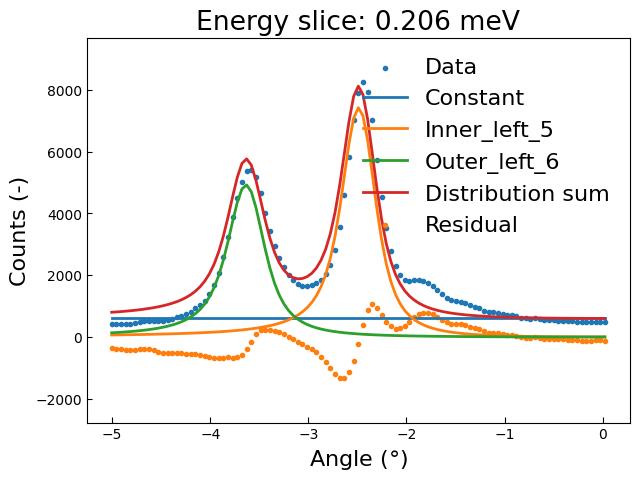
guess_dists = xarpes.CreateDistributions([
xarpes.Constant(offset=600),
xarpes.SpectralQuadratic(amplitude=3600, peak=-2.45, broadening=0.00024,
center_wavevector=k_0, name='Inner_left', index='5'),
xarpes.SpectralQuadratic(amplitude=1800, peak=-3.6, broadening=0.0004,
center_wavevector=k_0, name='Outer_left', index='6')
])
mat_el = lambda x: np.sin(np.deg2rad(x - theta_0)) ** 2
mat_args = {}
energy_range = [-0.1, 0.003]
angle_min=-5.0
angle_max=0.0
mdcs = xarpes.MDCs(*bmap.mdc_set(angle_min, angle_max, energy_range=energy_range))
fig = plt.figure(figsize=(7, 5)); ax = fig.gca()
fig = mdcs.visualize_guess(distributions=guess_dists, matrix_element=mat_el,
matrix_args=mat_args, energy_value=0.000, ax=ax)
[ ]:
%matplotlib widget

fig = plt.figure(figsize=(8, 6)); ax = fig.gca()

fig = mdcs.fit_selection(distributions=guess_dists, matrix_element=mat_el,
                         matrix_args=mat_args, ax=ax)

[ ]:
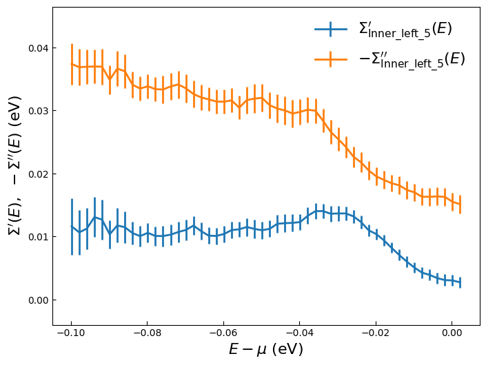
%matplotlib inline

fig = plt.figure(figsize=(8, 6)); ax = fig.gca()

self_five = xarpes.SelfEnergy(*mdcs.expose_parameters(select_label='Inner_left_5',
                                bare_mass=0.59521794, fermi_wavevector=0.141069758, side='left'))

self_six = xarpes.SelfEnergy(*mdcs.expose_parameters(select_label='Outer_left_6',
                                bare_mass=0.58997502, fermi_wavevector=0.1411192, side='left'))

fig = self_five.plot_both(ax=ax)
[ ]:
%matplotlib inline
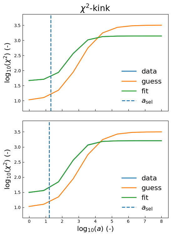
fig, ax = plt.subplots(2, 1, figsize=(6, 8))
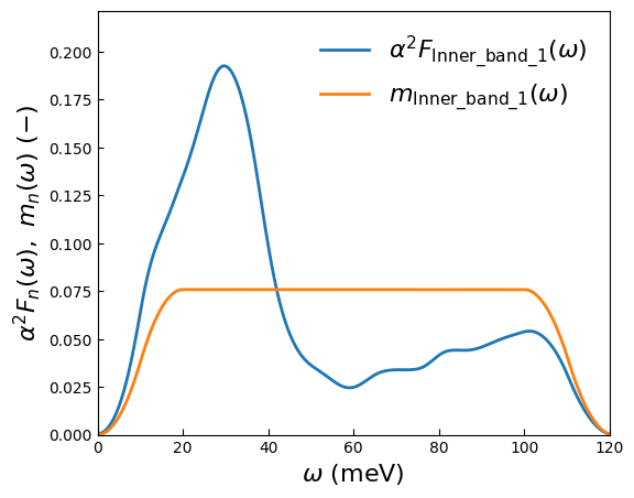
fig, spectrum, model, omega_range, aval_select = self_energy.extract_a2f(
omega_min=0.5, omega_max=120, omega_num=250,
omega_I=20, omega_M=100, omega_S=1.0, aval_min=0.0,
aval_max=8.0, aval_num=10, parts='both',
ecut_left=3.0, h_n=0.0741008, impurity_magnitude=16.475007,
ax=ax[0], show=False, fig_close=False)
fig, spectrum_left, model, omega_range, aval_select = self_five.extract_a2f(
omega_min=0.5, omega_max=120, omega_num=250,
omega_I=20, omega_M=100, omega_S=1.0, aval_min=0.0,
aval_max=8.0, aval_num=10, parts='both',
ecut_left=3.0, h_n=0.0743720, impurity_magnitude=15.882396,
ax=ax[1], show=False, fig_close=False)
# Figure customization
ax[0].set_xlabel(''); ax[0].set_xticklabels([])
ax[0].set_title('$\chi^2$-kink')
fig.subplots_adjust(top=0.92, hspace=0.1)
plt.show()
Dimensionality has been reduced from a matrix of rank 86 to 74 in the singular space.
Dimensionality has been reduced from a matrix of rank 86 to 74 in the singular space.
[ ]:
with xarpes.trim_notebook_output(print_lines=10):
    spectrum, model, omega_range, aval_select, cost, params = self_energy.bayesian_loop(omega_min=0.5,
                omega_max=120, omega_num=250, omega_I=20, omega_M=100, omega_S=1.0,
                aval_min=0.0, aval_max=8.0, aval_num=10, method='chi2kink',
                parts='both', ecut_left=3, iter_max=1e4, t_criterion=1e-8,
                power=4, bare_mass=0.6094394681, fermi_wavevector=0.1420916364, h_n=0.07582382627,
                impurity_magnitude=14.64962434, lambda_el=2.064840668e-07,
                vary=("impurity_magnitude", "lambda_el", "fermi_wavevector", "bare_mass",
                    "h_n"), scale_imp=1.0, scale_lambda_el=1.0, scale_kF=0.1, scale_mb=1.0, scale_hn=1.0)
Dimensionality has been reduced from a matrix of rank 86 to 74 in the singular space.
Iter    1 | cost = -2.7487e+02 | bare_mass=0.60943947 | fermi_wavevector=0.14209164 | h_n=0.075823826 | impurity_magnitude=14.649624 | lambda_el=2.0648407e-07
Iter    2 | cost = -2.7487e+02 | bare_mass=0.60943947 | fermi_wavevector=0.14209164 | h_n=0.075823826 | impurity_magnitude=14.649874 | lambda_el=2.0648407e-07
Iter    3 | cost = -2.7472e+02 | bare_mass=0.60943947 | fermi_wavevector=0.14209164 | h_n=0.075823826 | impurity_magnitude=14.649624 | lambda_el=0.00025020648
Iter    4 | cost = -2.7482e+02 | bare_mass=0.60943947 | fermi_wavevector=0.14211664 | h_n=0.075823826 | impurity_magnitude=14.649624 | lambda_el=2.0648407e-07
Iter    5 | cost = -2.7486e+02 | bare_mass=0.60968947 | fermi_wavevector=0.14209164 | h_n=0.075823826 | impurity_magnitude=14.649624 | lambda_el=2.0648407e-07
Iter    6 | cost = -2.7486e+02 | bare_mass=0.60943947 | fermi_wavevector=0.14209164 | h_n=0.076073826 | impurity_magnitude=14.649624 | lambda_el=2.0648407e-07
Iter    7 | cost = -2.7472e+02 | bare_mass=0.60953947 | fermi_wavevector=0.14210164 | h_n=0.075923826 | impurity_magnitude=14.649724 | lambda_el=0.00024979352
Iter    8 | cost = -2.7480e+02 | bare_mass=0.60946447 | fermi_wavevector=0.14209414 | h_n=0.075848826 | impurity_magnitude=14.649649 | lambda_el=0.00012520648
Iter    9 | cost = -2.7479e+02 | bare_mass=0.60951447 | fermi_wavevector=0.14209914 | h_n=0.075898826 | impurity_magnitude=14.649699 | lambda_el=0.00012479352
... (42 lines omitted) ...
Iter   52 | cost = -2.7487e+02 | bare_mass=0.60926944 | fermi_wavevector=0.14208995 | h_n=0.075834881 | impurity_magnitude=14.649764 | lambda_el=3.7040743e-07
Iter   53 | cost = -2.7487e+02 | bare_mass=0.60928633 | fermi_wavevector=0.14209048 | h_n=0.075833953 | impurity_magnitude=14.649744 | lambda_el=1.7570327e-07
Iter   54 | cost = -2.7487e+02 | bare_mass=0.60929518 | fermi_wavevector=0.1420921 | h_n=0.075862858 | impurity_magnitude=14.649606 | lambda_el=4.6761225e-07
Iter   55 | cost = -2.7487e+02 | bare_mass=0.6093019 | fermi_wavevector=0.14209057 | h_n=0.0758247 | impurity_magnitude=14.649762 | lambda_el=1.163109e-07
Iter   56 | cost = -2.7487e+02 | bare_mass=0.60925407 | fermi_wavevector=0.14208975 | h_n=0.075812797 | impurity_magnitude=14.6497 | lambda_el=2.3758286e-07
Iter   57 | cost = -2.7487e+02 | bare_mass=0.60931316 | fermi_wavevector=0.14209135 | h_n=0.075841729 | impurity_magnitude=14.649724 | lambda_el=1.2688221e-07
Iter   58 | cost = -2.7487e+02 | bare_mass=0.60928506 | fermi_wavevector=0.14208955 | h_n=0.075893389 | impurity_magnitude=14.649802 | lambda_el=4.298658e-08
Iter   59 | cost = -2.7487e+02 | bare_mass=0.60930009 | fermi_wavevector=0.1420913 | h_n=0.075816636 | impurity_magnitude=14.649693 | lambda_el=2.0686296e-08
Optimised parameters:
bare_mass=0.6093000865, fermi_wavevector=0.1420912972, h_n=0.07581663582, impurity_magnitude=14.64969312, lambda_el=2.068629643e-08
[ ]:
%matplotlib inline

fig = plt.figure(figsize=(6, 5)); ax = fig.gca()

fig = self_energy.plot_spectra(ax=ax)

plt.show()